Restaurant – Jake Starkey

##Question 1

library(tidyverse)
library(skimr)

Load the data.frame for Question 1.

restaurant <- read.csv('https://bcdanl.github.io/data/DOHMH_NYC_Restaurant_Inspection.csv')

Q1a

What are the mean, standard deviation, first quartile, median, third quartile, and maximum of SCORE for each GRADE of restaurants?

restaurant %>% 
  group_by(GRADE) %>% 
  skim(SCORE) %>% 
  select(-n_missing)

Data summary
Name	Piped data
Number of rows	17633
Number of columns	12
_______________________
Column type frequency:
numeric	1
________________________
Group variables	GRADE

Variable type: numeric

skim_variable	GRADE	complete_rate	mean	sd	p25	p50	p75	p100	hist
SCORE	A	1	9.26	3.42	7	10	12	13	▁▂▂▅▇
SCORE	B	1	21.03	4.16	18	21	24	36	▁▁▇▇▁
SCORE	C	1	38.56	10.83	31	36	44	86	▁▇▇▂▁

Q1b

How many restaurants with a GRADE of A are there in NYC? How much percentage of restaurants in NYC are a GRADE of C?

freq <- as.data.frame( table(restaurant$GRADE) )

prop <- as.data.frame( 100 * prop.table(table(restaurant$GRADE)) )

Q1c

Provide both (1) ggplot code and (2) a simple comment to describe how the distribution of SCORE varies by GRADE and CRITICAL FLAG.

Boxplots

ggplot(restaurant) +
  geom_boxplot(aes(x = SCORE, y = GRADE, fill = GRADE) ) +
  facet_grid( CRITICAL.FLAG ~ . )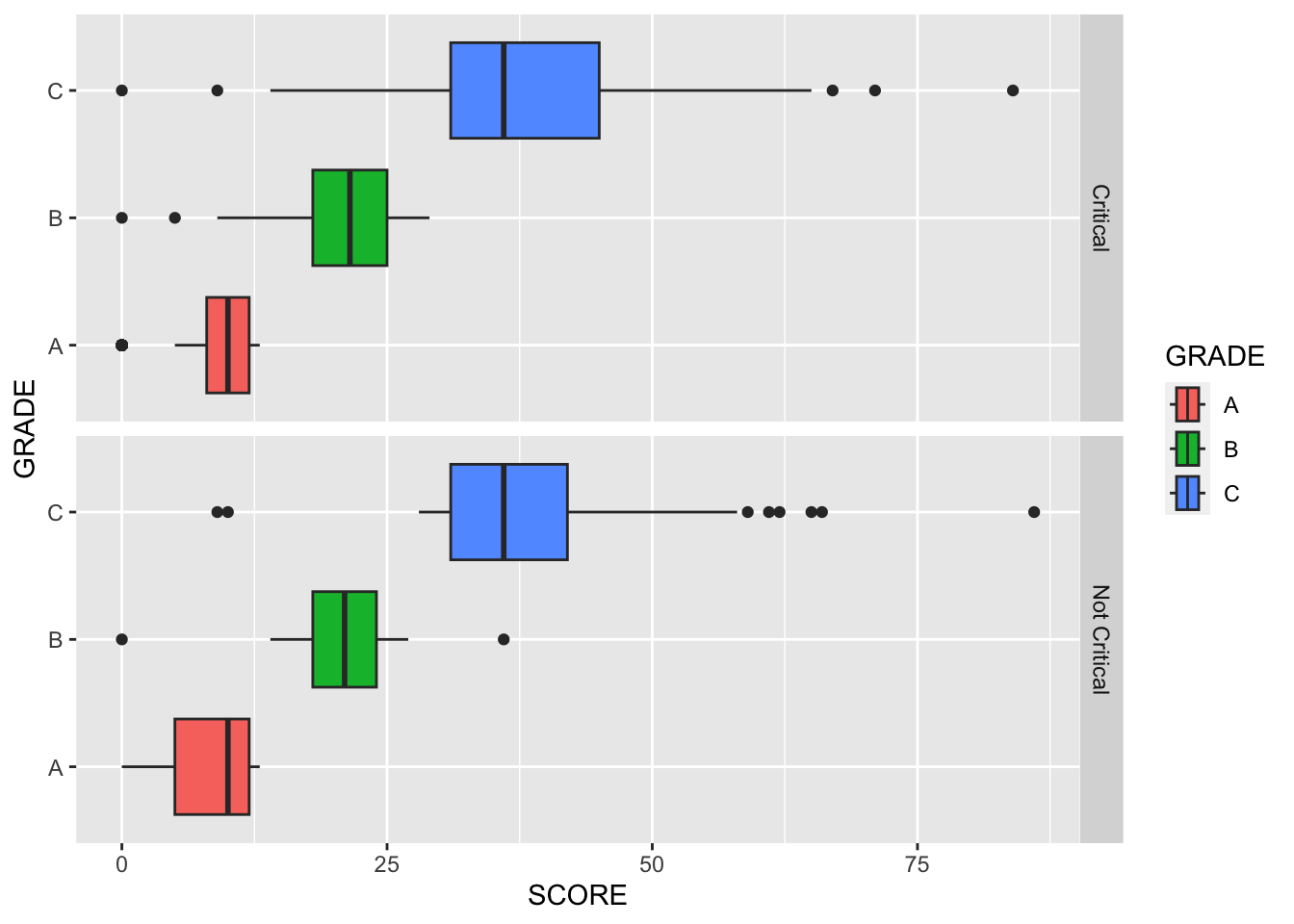

-Histograms

ggplot(restaurant) +
  geom_histogram(aes(x = SCORE), binwidth = 1 ) +
  facet_grid( CRITICAL.FLAG ~ GRADE )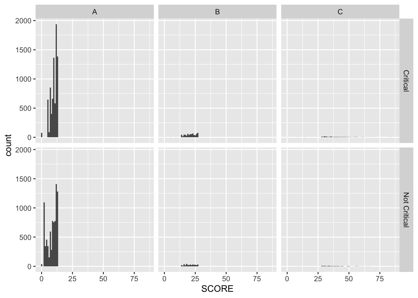

-Mostly, -The values of SCORE for GRADE A ranges from 0 to 13. -The values of SCORE for GRADE B ranges 13 to 27. -The values of SCORE for GRADE C ranges 24 to 75. -For Not Critical type, two SCORE values around 1 and 12 are most common, while 12 is the single most common SCORE value for Critical type.

Q1d

Provide both (1) ggplot code and (2) a simple comment to describe how the proportion of CRITICAL FLAG varies by GRADE and BORO.

ggplot(restaurant) +
  geom_bar(aes(x = CRITICAL.FLAG,
               y = after_stat(prop), group = 1)) +
  facet_grid( GRADE ~ BORO )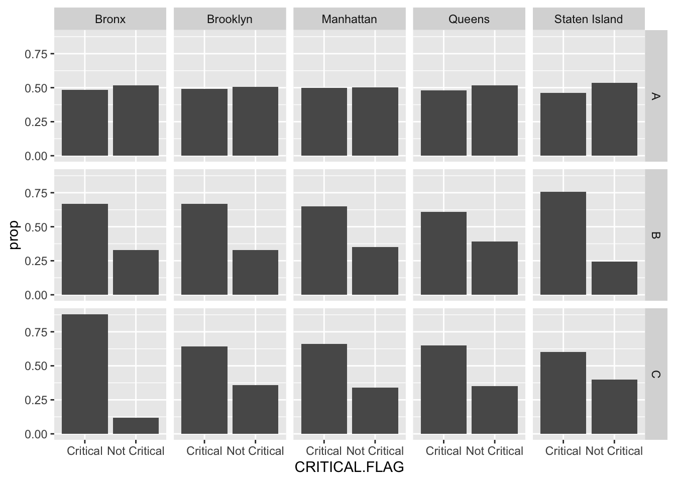

-For GRADE A, the probability distribution of CRITICAL FLAG are similar across BOROs.

-For GRADE B, the restaurants in Staten Island are more likely to be Critical than in other BOROs.

-For GRADE C, the restaurants in Bronx are more likely to be Critical than in other BOROs.

Q1e

For the 10 most common CUISINE DESCRIPTION values, find the CUISINE DESCRIPTION value that has the highest proportion of GRADE A.

q2e <- restaurant %>% 
  group_by(CUISINE.DESCRIPTION) %>% 
  mutate(n = n()) %>% 
  ungroup() %>% 
  filter(dense_rank(-n) <= 10) %>% 
  group_by(CUISINE.DESCRIPTION, GRADE) %>% 
  count() %>% 
  group_by(CUISINE.DESCRIPTION) %>% 
  mutate(prop_A = n / sum(n)) %>% 
  filter(GRADE == 'A') %>% 
  arrange(-prop_A)

Q1f

-Find the 3 most common names of restaurants (DBA) in each BORO. -If the third most common DBA values are multiple, please include all the DBA values. -Overall, which DBA value is most common in NYC?

q2f <- restaurant %>% 
  select(DBA, BORO) %>% 
  group_by(BORO, DBA) %>% 
  summarize(n = n()) %>% 
  mutate(ranking = dense_rank(-n)) %>% 
  filter(ranking <= 3) %>% 
  arrange(BORO, ranking)

q2f_ <- restaurant %>% 
  group_by(DBA) %>% 
  count() %>% 
  arrange(-n)

Note that chipotle mexican grill and subway are both the third most popular franchise/chain in Manhattan. 🌯

Overall, dunkin is the most popular franchise/chain in NYC. 🍩

Q1g

For all the DBA values that appear in the result of Q1f, find the DBA value that is most likely to commit critical violation.

q2g <- restaurant %>% 
  filter(DBA %in% q2f$DBA) %>% 
  group_by(DBA, CRITICAL.FLAG) %>% 
  count() %>% 
  group_by(DBA) %>% 
  mutate(lag_n = lag(n),
         tot = sum(n),
         prop_crit = lag_n / tot) %>% 
  select(DBA, prop_crit) %>% 
  filter(!is.na(prop_crit)) %>% 
  arrange(-prop_crit)

-Among popular franchises/chains, subway is most likely to commit Critical violation in NYC. 🥪